")

Actual performance & risks
The risks of Index Investing on Wall Street
An investor runs a market risk on his stock investments, because the values of his investments appear to fluctuate randomly. During economic downturns, the fluctuations appear to add up downwards to a so-called Maximum Drawdown (MDD). The MDD is a good measure for the maximum interim loss an investor may suffer on his long-term expected annualized return. During upturns, the fluctuations appear to add up to new heights. DigiFundManager introduces the concept of a validation period, a period of "Out-Of-Sample" testing of actual historic cumulative value fluctuations of the calculated time series of portfolios. We optimize the weightings in a gradient search to get optimal portfolios. We try to make sure that the back test in hindsight represents the actual value fluctuations of the investments over time, including stocks that have become inactive. We advise the user to extend the validation period as to include at least the last Global Financial Crisis (GFC), at least 15 years, preferably 30 years. Stock Indices (S&P500 and the DJIA) are known to go down by about -50% during recessions. Not only retail investors cannot bear intermediate losses of -50% on long-term annualized gains of 7%-8%:
- Large drawdowns on the way to a long-term average can leave you without means to live your life.
- Several banks went broke or needed and received financial injections on their ways to long-term averages during the last financial crisis as they were too big to fail.
DigiFundManager uses the Risk-Reward-Ratio (RRR) as a number to represent the balance between your investment at risk and your expected annualized result. We take the absolute value of the MDD as the Risk, and for the Reward we take the annualized results, both over the validation period. Professionals may be better acquainted with the MAR ratio or indicator, which equals the inverse of the RRR. For Indices, RRR ≈ 6 - 8, so that the maximum interim value at risk is on the order of half of your investment when the annualized reward is of the order of 7%-8%. By using hedging and statistical techniques like the one developed by Markowitz, one may be able to reduce the RRR from ≈ 6 - 8 to a more balanced value of about 1 to 0.5 of properly screened and ranked portfolios.
The drawdown of -10% of October 2018 and of -19% in December 2018
October 2018 was known for a -10% downturn of the S&P500. My own investment at the time was an optimal portfolio with 12 long positions hedged by 12 short positions purchased on September 27 for 13 weeks calculated by DigiFundManager. The weighting was calculated using the Markowitz technique with the RRR as the objective function rather than the variance of the results. With hedging and the Markowitz technique in action, we statistically expect an annualized reward of 16% validated ("out-of-Sample" testing) over 30 years with an MDD of -11% after costs (black curve):

These simulated results showed YTD = 15% at the end of the scan on 26-Sep-18. My broker showed the following eod value fluctuations of my portfolio (green-red curve in Euros) over October 2018 with the S&P500 as benchmark (blue curve):

Statistics do not give you any guarantee for future performance. The mathematician and alma mater of the quantitative investment strategies, Jim Simons, stated in 2005 that past performance is the best predictor of success. Expectation values are calculated from past performance. They may indicate an increase of your chances on future success when the nature of risks does not change as shown by these empirical results obtained by trading on Wall Street.
Nassim Taleb's black swan
When the nature of risks does change but is not recognizable in mathematical correlations of the past, we arrive at the area of Nassim Taleb. He formulates unrecognizable stions. DigiFundManager minimizes the maximum drawdown divided by the annualized result as one of three options hapes of randomness, the so-called black swans, that are supposedly residing in the tail of the distribution funcfor a given set of correlation times. That implies a search of an optimization process in the tail of a distribution function. When such numerical correlation processes are mathematically unrecognizable, the effectiveness of quantitative strategies should break down for such shapes.
Markowitz and hedging in action
I rebalanced my long portfolio on 22 April 2024, as calculated by the program. Since September 26, 2018, my account in Dollars gained +43.5%, including costs, with an MDD of -47.1%, while the S&P500 [$] went up by +73.7% with an MDD of -34%. Indeed, Markowitz and hedging in action. Below you see the actual eod performance in Dollars of my broker account since 26 September 2018 (white curve), including costs and compared to the S&P500 [$]:
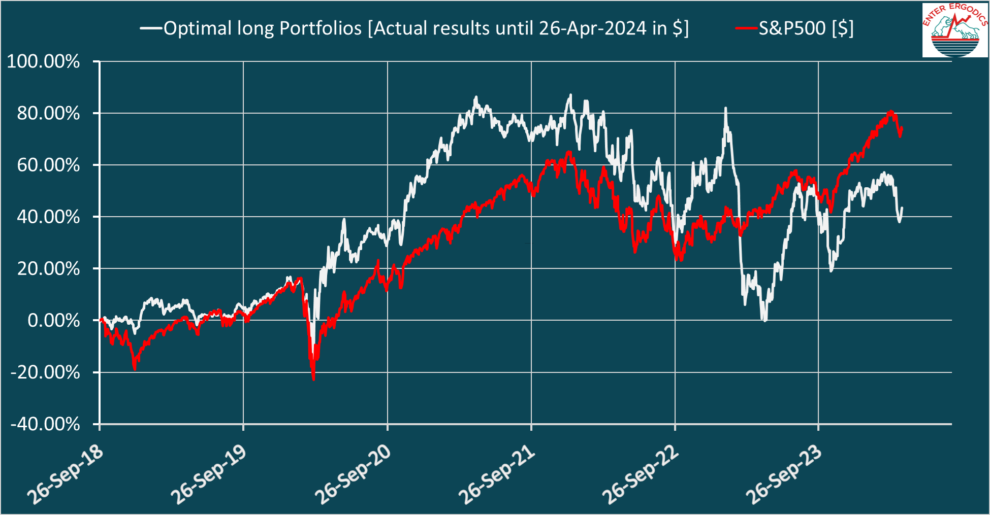
In 2024, the YTD [$] results are -3.7% versus +5.8% of the S&P500.
The efficient-market hypothesis and the search for autocorrelations
With the continuous stream of financial, political, and economic information, one usually tries to compose, weight, and maintain stock portfolios with maximized returns and minimized risks. One often assumes the efficient-market hypothesis (EMH). This hypothesis implies that asset prices always reflect all available public information, suggesting that historical asset prices are all you need to compute optimal portfolios. Our software only uses historical eod exchange data and confirms this view. That does not mean that you cannot beat indices such as the S&P500. It does mean that share prices are right, so that you can statistically predict in which direction they will move. You may time those predictions using the Wiener-Khinchin-Einstein theorem. This theorem enables you to search for the market timing (holding periods) with the strongest autocorrelations in the portfolio-value fluctuations over economic upturns and downturns. Hence, the price movements of the past enable you to compute your best predictor of future success. That is what quantitative strategies strive for. Hedge funds like Bridgewater, D. E. Shaw and Renaissance, all three achieved double-digit results over 2018, while on average the industry made about -5% compared to -6.2% of the S&P500. All three used, at least partly, quantitative strategies. DigiFundManager shows that such top results were indeed possible, be it for smaller investments that fit retail investors and only using historical end-of-day stock prices, volumes, dividends, and splits.
MiFid2 rulings for PRIIPs products on quantitative risk assessment
MiFid stands for Markets in Financial Instruments Directive for the European Union, and PRIIPs stands for Packaged Retail and Insurance-based Investment Products. These products include ETFs, investment funds, and funds of funds. MiFid2 rulings for PRIIPS products literally state that "Market risk is measured by the annualised volatility corresponding to the value-at-risk (VaR) at a confidence level of 97,5 % over the recommended holding period, unless stated otherwise. The VaR is the percentage of the amount invested, that is returned to the retail investor." The market party that delivers the PRIIPs product is required to calculate the Var-equivalent volatility (VEV) and assign a Market Risk Measure (MRM) class. This MRM class needs to be combined with other Credit Risk Measures (CRM), if present, and then translated into a number, the so-called Risk Indicator (RI). The MiFid2 risk indicator for PRIIPs products can assume a value between 1 and 7. For example, when the VEV lies between 20% - 30%, the RI or MMR class assume the value of 5 when other risks are not significantly present:

PRIIPs products are divided into four categories.
One scan over historical value fluctuations tells you more than 10,000 sets of fictitious fluctuations
Risks and annualized results are calculated from a minimum of 10,000 selections of fictitious fluctuations for Category 3 products. It is like drawings from a lottery. Neyman was the one who introduced confidence intervals. He already warned for the fact that a confidence interval (here 97.5%) only bears information about the value of the drawings and about the reliability of the drawing process. Such a drawing process bears no information about historic quantities like expected results and risks on those results. To state that these fictitious value fluctuations have anything to do with real historical quantities is considered as a misunderstanding according to Wikipedia. You simply cannot determine real historic value fluctuations from 10,000 fictitious fluctuations. According to us, the calculation of a VaR-equivalent volatility (VEV) on the basis of a fictitious history cannot be applied to formulate an ex-post risk indicator. Monte Carlo simulations are generally applied in signal processing, where the propagation of signals in the future is determined by laws of physics. But the propagation of exchange prices is fundamentally unpredictable. That is why we calculate the expected annualized result and maximum interim loss of realistic portfolios from clean historical data.
Risks calculated from volatility versus risks calculated from maximum drawdowns
We believe that the calculation of the VEV makes the problem unnecessary complicated. A retail investor typically wants to know his maximum interim loss on his expected reward for his time horizon. DigiFundManager introduces the ratio of the two as the Risk/Reward ratio. Focus is on to get this ratio to about “1”, hence as small as possible. In the professional investment world, one often works with a kind of average risk. One takes the volatility as this average risk. Volatility is calculated as the standard deviation over the time horizon on the basis of given holding periods. This average risk is often a factor of three to four smaller than the maximum interim loss. Volatility as a risk measure works 80% of the time, "but not when you need it most, when tail events kick in". In Modern Portfolio Theory (MPT), the so-called MPT-statistics are formulated. The standard deviation (= volatility) is an example of such statistics. Other statistical quantities that are often included in a risk analysis are the Sharpe ratio (Reward/Average-Risk ratio relative to the S&P500), beta (risk relative to the S&P500 minus the risk-free rate of 10Y US bonds), and alpha (the annualized reward minus the risk-free rate relative to the risk-adjusted S&P500 minus the risk-free rate). In our free online version, we calculate these MPT-statistics and the risk indicator.
The risk profile of the S&P500
Portfolios of non-penny stocks with sufficient daily trading liquidity without "Over-The-Counter" (OTC) stocks suffer barely from any credit risk. For such stocks, the main risk is the market risk. As an example, consider the annualized results of weekly trading the S&P500. These annualized results vary by a factor of two when the validation period decreases from 68 years to 5 years. The skew increases by a factor of two, and kurtosis varies by a factor of four. The annualized volatility varies between 12% and 18%. Hence, the sequence of weekly results of the S&P500 cannot just be randomized to calculate a practical value at risk. Only the real sequence gives you a mean with an MDD as a practical risk level. This population mean can be considered as an expectation value when the weightings of the stocks in each portfolio are normalized to one. For compounded investments, the MDD = -56% for validation periods between 68 and 12 years. For constant investments, the corresponding number is -75%. These are your risk levels when you are involved with Index investing. According to us, the RI of the MiFid2 rulings for Category-3 PRIIPs products bears no formal relevance to chances on risks and rewards.
How does your market risk scale with (equivalent) volatility?
For a given annualized volatility, σa, validation period, Nval, and Clément Juglar (1862) investment cycle, Ninv, it is mathematically straightforward to proof the existence of a minimum Value-at-Risk determined by the inequality:
VaR ≥ (Nval/2Ninv)σa.
Mathematics is no physics or finance. It does not have to comply with the real world. An investment cycle encompasses a period of economic growth followed by a period of economic contraction and lasts about 7-11 years. When the validation period contains two of those investment cycles, which adds up to about 20 years, the mathematical minimum of the Value-at-Risk equals the volatility. For a median pick out of [12%, 17%], your market risk, or your Value-at-Risk would then be 14.5% of your investment with your Risk-Indicator on 5. But does that give a realistic view of the situation? Indeed, we know from Index investing that the practical Value-at-Risk is about a factor of 3.5 higher. Therefore, it may be misleading to equate the market risk with volatility.
Jan G. Dil and Nico C. J. A. van Hijningen,
Apr 26, 2024.